When to Replace Orca Bushings

• Introduction

The maintenance cycle of the Orca™ Series motors may be of great importance to a select few applications, particularly those in factory settings with considerable side load. The exact service life of the bushings is entirely dependent upon the loading characteristics of the application, and some loading conditions never require bushing replacement. Fortunately, IGUS provides a calculator on the life cycle for the bushings in the motors.

The mechanical interface between stator and the shaft is a thin plain flanged bushing. The IGUS product code is GFM-2526-25. This bushing has a wall of 0.5mm thick, which accommodates the cutting edge force efficiency of these motors.

This article will teach how to find the life cycle of the bushings using the IGUS Calculator. 

• Bushing Size and Loading Characteristics

The first page of the Igus Calculator can be found annotated below:

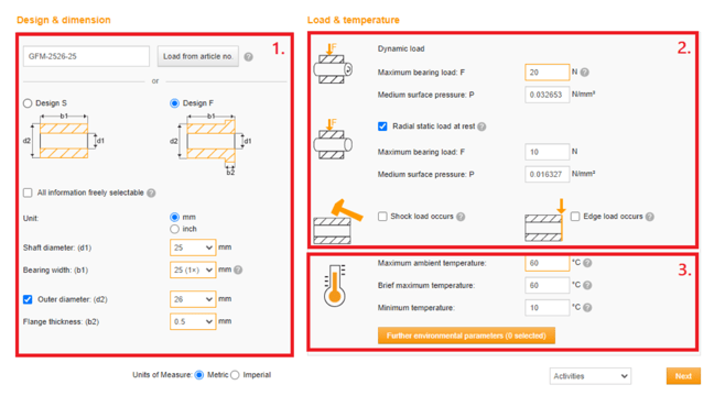
1. The bushing Size is automatically filled in by typing “GFM-2526-25” into the article number box and loading the parameters.
2. There are two bushings in an Orca Series motor, the data for the Loading should be considered for the worst case bushing. The dynamic loading of the motor is dependent on the location of the load and the application orientation. Two common loading cases can be found here:

• The shaft is supported by both sides

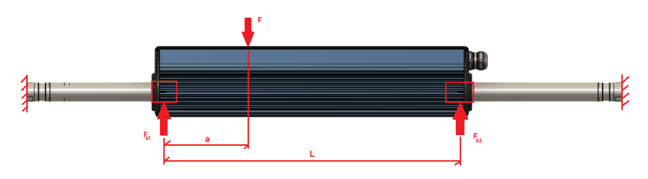
In this case, the bushing side load is entirely dependent upon the location of the force on the side of the stator, and the length of the shaft has no effect on the side loads. The equations for the bearing side loads are as follows:

F_b1=F-aF/L                             F_b2=aF/L

Where F is the side load of a motor simplified to a point load, this may have to be calculated from an aggregate of different loads. a is the location of the force from the first bushing, and L is the spacing of the bushings, from center point to center point. This is dependent on the length of the Stator. The following table shows these lengths for each stator type:

So as an example, if 100N was place on an Orca-6 at 70mm from the first bushing:

F_b1=100N-70mm*100N-156.9mm=55.39N                     F_b2=70mm*100N/156.9mm=44.61N

• The shaft is supported with the cantilever of the bushing

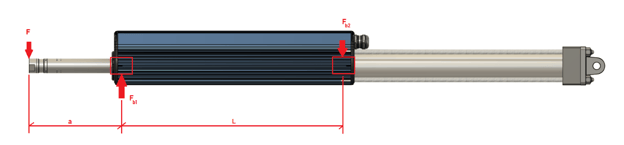
In this case, the bearing load is now dependent on the length and position of a shaft, this is the use case that amplifies the exerted force onto the bushings. The equations for the bearing side load is as follows:

Fb1 = F + aF/L                             Fb2 = aF/L

Where F is the side load of a motor simplified to a point load, this may have to be calculated from an aggregate of different loads. a is the location of the force on the shaft measured from the centre point of the first bushing, and L is the spacing of the bushings, from centre point to centre point. This is dependent on the length of the stator. Table 1 contains the values of the bearing spacing.

It’s important to note that a is not equal to the shaft throw, and it does not measure from the end of the stator. The distance from the centre of the bushing to the end of the stator is 12.5mm. 

It’s also important to note that Iris Dynamics recommends supporting lateral loads with linear bearings to reduce friction and increase the life cycle of the bushings.

1. The temperatures of the application site should be the worst case scenario. The brief maximum temperature can be set to 70 degrees.

• Motion Profiles

The next page of the calculator focuses on the motion type and profile. A motor with minor and slow movements will maintain healthy bearings longer than the same motor undergoing larger and quicker motions. The annotated page can be found below:

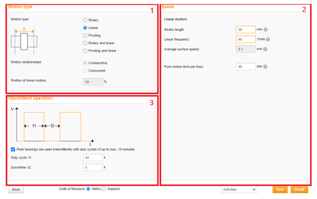
1. The Motion Type should either be “linear” or “rotary and linear” depending on the application. Most applications will only be linear.
2. The important value in this box is the average speed. Due to the nature of a linear motor being one of constant starting and stopping, this part of the calculator requires some formulas. First is the travel of motion, using kinematic profiles as opposed to other control methods:
   
   Stroke = i = 0kxi 
   
   Where this is the sum of all of the delta positions of the motions in the kinematic profile. This is the full distance the motor travels in one cycle. Use the worst case scenario.
   
   Time = i = 0kti + Delayi
   
   Where this is the sum of all kinematic motions and position delays in seconds. The worst case scenario for this is the lowest time to complete a cycle.
   
   Linear Frequency = 60s / Time
   
   A 1Hz kinematic profile would have a linear frequency of 60/min. Finally, the pure motion time per hour can be calculated:
   
   Pure Motion Time per Hour = 60min * i = 0kti / Time
   
   This is the ratio of kinematic motion time to full profile time multiplied to 60 minutes.
3.  Intermittent operation is an optional addition. The time delays of positions can be added into the calculator in pure motion time per hour from above, though if there are pauses between individual profiles they can be outlined here.

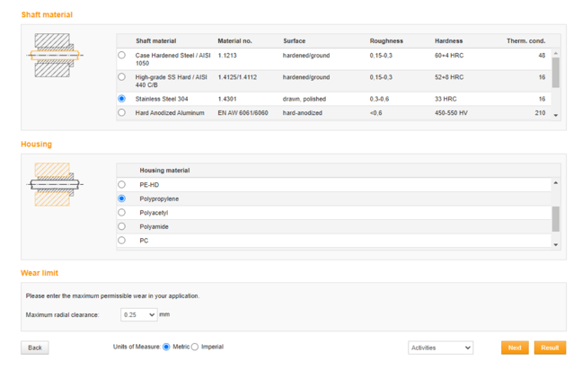
• Materials and Wear Limits

The final page for variable entry selects the housing and shaft materials. The Housing is a glass filled Polypropylene, the shaft is 304 Stainless Steel, and the recommended wear limit is 0.25mm.

• Bushing Results

After filling the data from the previous pages, it is now possible to find the bushing lifetime. The bushings are G300. The service life can then be determined. The corresponding number of cycles can be found by reverse calculating using the variables on the Motion Page.

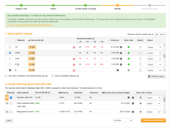
The accurate service life is entirely dependent on a comprehensive use case analysis. The full life of a bearing may only be realized with clean surfaces, free of excess humidity and excess heat. This calculation can provide valuable estimations on the effect of load and motion on the maintenance cycle.