- November 24, 2022
Feature Highlight: Kinematic Controller
ORCA™ Series Motors Kinematic Controller Highlights
Introduction
Derived from the Greek kinema (“movement”), Kinematics is a branch of physics which aims to describe the motion of objects. If the initial conditions are known, we can use equations of motion to predict how a given object will move.
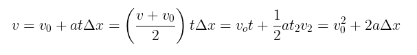
Think back to science class: if you throw a ball upwards at a known velocity, how high does it go before gravity begins to bring it back down? How much faster do you have to throw it to reach twice that height? These are questions we can answer with the familiar basic kinematic equations:
ORCA Series linear motors come equipped with a kinematic controller which can generate shaft motion profiles given a target position and a travel time. In the example problem from earlier, the ball is under the constant acceleration of gravity, therefore the simple kinematic equations sufficed. But what if acceleration is a variable we are interested in controlling?
To achieve the point-to-point shaft motion that requires the least amount of power, a linearly varying acceleration is ideal. Using the constraints along with linear algebra techniques, it is possible to derive a function of position over time. From there, the ORCA Series motor’s position controller can take over and drive the shaft to follow that path.
Let’s look at the mathematics behind how the ORCA Series achieves one of the available kinematic motion types: linear acceleration.
Significance
Industrial automation uses linear motion extensively, and often this is done with rudimentary controls such as two-state pneumatic cylinders. Often the control that an automation engineer has over their device is “go” and “return.” While this is often enough to get the job done – at least initially – changing process variables, environmental conditions, and component age will affect what actually happens when “go” or “return” is commanded.
The result is often that a system that worked when commissioned begins to fail or result in compromised quality and throughput later in its life. Or, sometimes the motion that results from “go” and “return” isn’t sufficiently graceful for the application.
A device that follows a kinematic path accommodates changing environments, process variables and component age, and maintains repeatability. It can also be tuned in many ways primitive controls cannot, which enables tighter timings on assembly lines and more precise control over products. For these reasons, it makes a lot of sense for an intelligent motor system to implement some form of kinematic controller.
Linear Acceleration Derivation
First, acceleration is defined to be a straight line using the generic linear function form of y=mx+b.
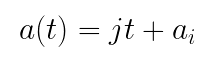
In this case, the symbol j is used to represent jerk, the rate of change or slope of acceleration. This will become more relevant later for the second type of kinematic motion.
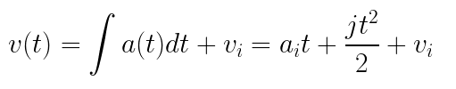
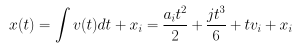
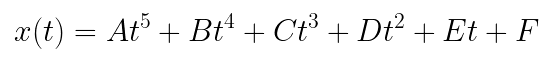
The functions for velocity and position are defined as the first and second integrals, respectively, of the acceleration equation.
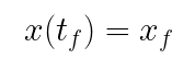
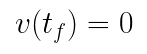
The conditions for the final position and velocity are known quantities. That final position is trivial as it is an input to the system. For velocity, the ORCA Series motor’s shaft should be fully stopped at the final position, so the final velocity will be 0.
With this information, the line the acceleration must lie upon can be solved for. The equations are put into a matrix and converted to reduced row echelon form to extract the solutions for j and a_t, and by extension the solution to the acceleration line.
There are now only two unknowns remaining to solve the final position equation: initial velocity (v_i), and initial position (x_i).
Thankfully, ORCA Series motors feature highly accurate sensors to provide this information. Armed with that data, the equations for jerk (j) and the initial acceleration (a_i) are now entirely described in terms of known variables.
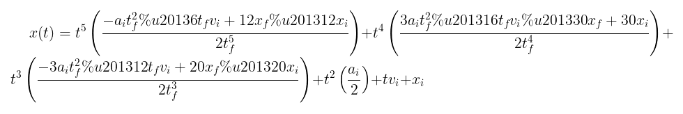
A fully solved equation for acceleration also brings a fully solved equation for position, by way of the integral definition from above. Below is the final simplified equation after substitution.
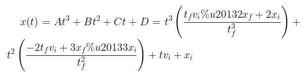
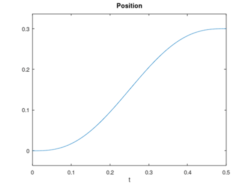
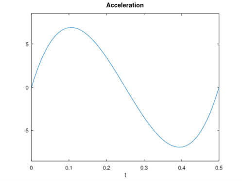
When initiating a motion, the coefficients of time are calculated and then each position step is calculated by passing the time since beginning the motion into the position function. Below is an example of the position and acceleration of a 300 mm motion over 500 ms.
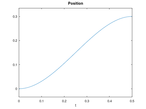
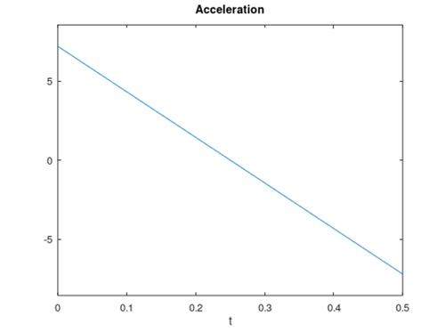
Position vs Time with Linear Acceleration Acceleration vs Time with Linear Acceleration
Minimum Jerk Derivation
If smooth motion is valued over minimal power consumption, the desired position path is one that experiences minimum total jerk over the course of the movement. In other words, the “cost” of the jerk function is minimized. It turns out that this is a relatively simple condition. The jerk cost of a position function is minimized when the sixth derivative is 0. Therefore, a general solution simply looks like this:
Working in the opposite direction from the linear acceleration derivation, the position equation can be differentiated twice to find v(t) and a(t). Adding in the initial conditions and solving the matrix gives equations for each coefficient in the polynomial x(t).
Notice that unlike the case where the constraint is linear acceleration, the position coefficients require a known initial acceleration. This value is available from the ORCA Series registers just like the position and velocity values.
Below is the position and acceleration output with the same 300 mm travel and 500 ms duration. Notice that the acceleration changes smoothly throughout the movement, as opposed to the linear acceleration profile which attempts to instantly reach an initial acceleration.
Position vs Time with Minimum Jerk Acceleration vs Time with Minimum Jerk
Using the Kinematic Controller
Setting up an ORCA Series motor to perform custom motion profiles is made easy with the IrisControls companion application. Connecting to an ORCA Series motor with a USB cable gives access to a full graphical user interface that includes a kinematic controller configuration page.
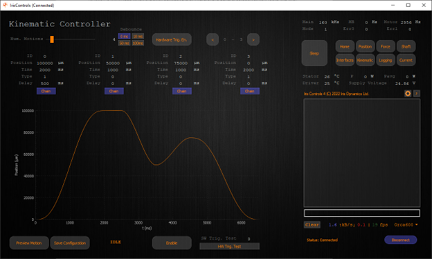
A Screenshot of the Kinematic Controller GUI for ORCA Series Linear Motors
Use this interface to configure and preview an ORCA Series motor’s motion profile and save it to permanent memory with a click of a button.
Motions can be triggered individually over the MODBUS serial protocol or from external hardware. Motions may also be chained together to create more complex or infinitely looping profiles.
Find more information on how to configure motions in the ORCA Series Motor Reference Manual.